Introducing Arrugator
TL;DR: I have made a very-purpose-specific javascript library to reproject GIS raster images using WebGL triangles.
One of the woes of being a polyglot is knowing the word for something in a foreign language, but not knowing the translation to one’s mother tongue, because there’s no good translation.
Such is the case with the word warp, specially in GIS contexts. It’s dictionary meaning is on point:
to turn or twist out of or as if out of shape especially: to twist or bend out of a plane
Every person in the GIS realm (that I know) hits, sooner or later, a dreadful nemesis: CRSs and map projections. The process of changing a map to a different CRS is known in the jargon as warping the map. Heck, the reference tool for this is called “gdalwarp”.
Using the word warp for maps makes sense: one can think of the map as a flat planar entity, and using a different CRS forces it to be bent out of the orginal plane. The word just has a precise topological meaning that hits the spot.
The Spanish translations of “warp” don’t cut it, though:
- “Combar” is used in carpentry and forestry contexts when wood gets bent out of shape (mainly) due to weather or humidity, or when talking about elastically bending sheet-like pieces of metal.
- “Encorvar” evokes images of elderly people hunched on walking canes, and of every time your parents reminded you that sitting so many hours in front of a computer screen is not good for your spine.
- “Alabear” is used in aeronautical contexts to denote the rotation of the plane along its longitudinal axis.
- “Deformar” implies losing form/shape.
- “Torcer” implies twisting, not having planar topology.
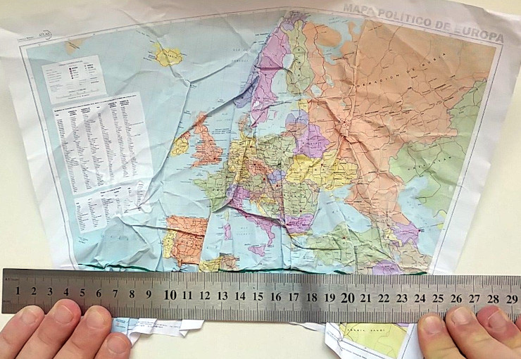
In my brain, none of those words works for maps. I’ll illustrate with a conical de-projection. First, I physically visualize the fitness of the cone:

I’m using a 1:10.000.000-scale political map of Europe, in Lambert equifeline conical projection (available at the download centre of the Spanish Geographical Institute). Interestingly enough, the 55th parallel of a fits perfectly on the outer edge of the cone of shame for veterinarian use conical scaffolfing unit when the map is printed on a A4 sheet of paper.

The fit is almost purrfect, save for a near-invisible deformation near the strip of sticky tape attachment point near Iceland.
Now, if I try to straighten up the 35th parallel, this happens:
That’s what my brain thinks when I’m “warping” a map: I crumple and rumple and wrinkle them. If “crumple” is «to press, bend, or crush out of shape», then, yes, reprojecting a map is akin to pressing it against a (planar) surface so they kinda fit in that new surface.
That’s why I like the Spanish translation of that concept: Arrugar.
I have been working on a tool do just that to maps, and an a flashy display of anglo-castilianist portmanteau-ing, I’v decided to call that tool arrugator.
It should be no secret that I’ve been working on tightening the capabilities of WebGL with the neccesities of the GIS field. Display of reprojected raster images is such a use case: it’s pure graphics manipulation (that’s what OpenGL/WebGL does) that is needed often in some applications. Furthermore, since I’m a Leaflet maintainer (even though 2020 has gotten in the way of working on Leaflet’s code base), one of the things I’m most jealous of OpenLayers is its raster reprojection capabilities.
Since I have been working on the OpenLayers code base lately, and with raster images on different projections to boot, I’ve seen the OpenLayers “dynamic iterative triangulation” diagram a lot of times:
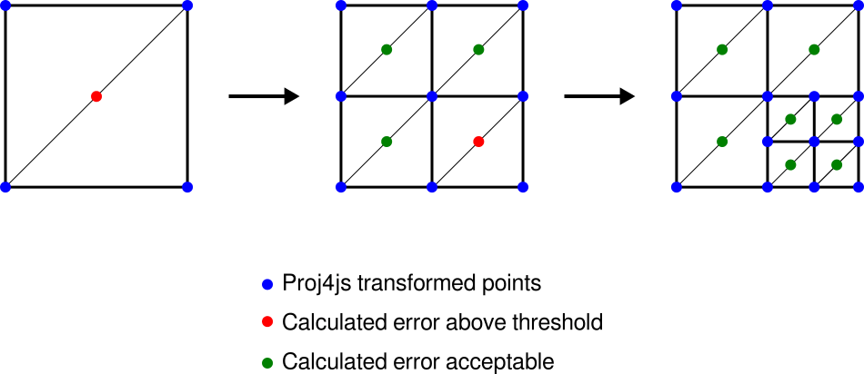
I don’t know exactly when, but my brain focused on those three points at the edge of a subdivision and started telling me: «There’s a sliver in there». It’s one of those OCD-like things I can’t unsee, ever.
Dammit, brain.
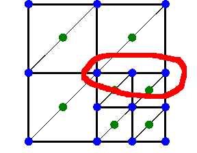
I haven’t been able to look at that diagram again and not see a supposedly-zero-area triangular sliver in those three points. This was before I realized that OpenLayers uses inverse reprojection, so that the square grid is actually square in the display projection, but nonetheless there’s gonna be a subpixel misalignment in there (or so I see it).
And then, I don’t know exactly when, I had a breakthrough (or, as we Spaniards say, a «happy idea»). Instead of a sliver-prone square grid, I could have a topologically nice triangular mesh; and instead of subdividing squares based on the length of the diagonal (which is what the OpenLayers diagram kinda shows), it should be possible to subdivide triangles instead, by the midpoints of their edges, starting with the edge with the greatest (estimated) error.
The “estimated error of a edge segment” is defined as the distance between:
- The midpoint of the segment defined by the projected endpoints, and
- The projected midpoint of the segment defined by the endpoints.
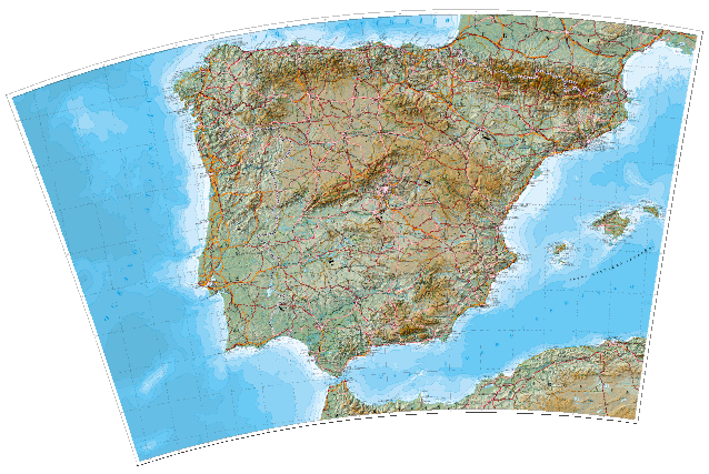
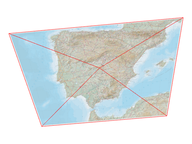
This is better explained with an example. I’m gonna use the 1:2million physical raster map from the Spanish Geographical Institute for illustrative purposes (available under a CreativeCommons-by-compatible license in their download centre). The original raster is in EPSG:25830 AKA “ETRS89 UTM30N”, like so:
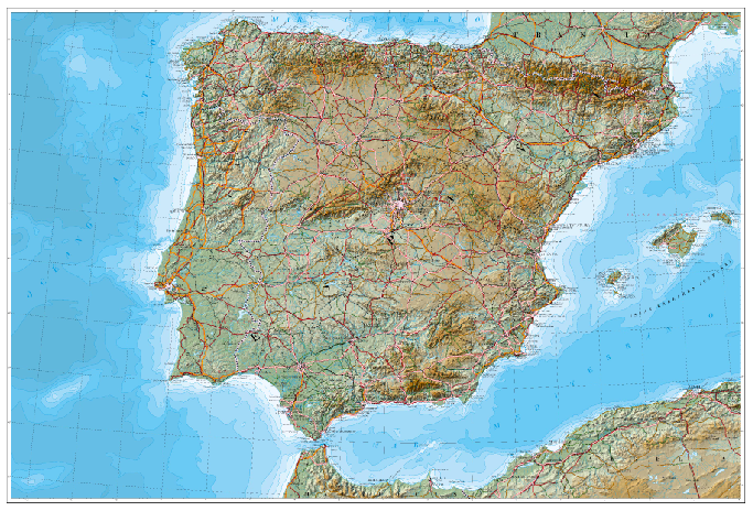
Now let’s warp crumple that map that into something showing an obvious distortion, such as EPSG:3031 AKA “WGS84 Anctartic Polar Stereographic”:
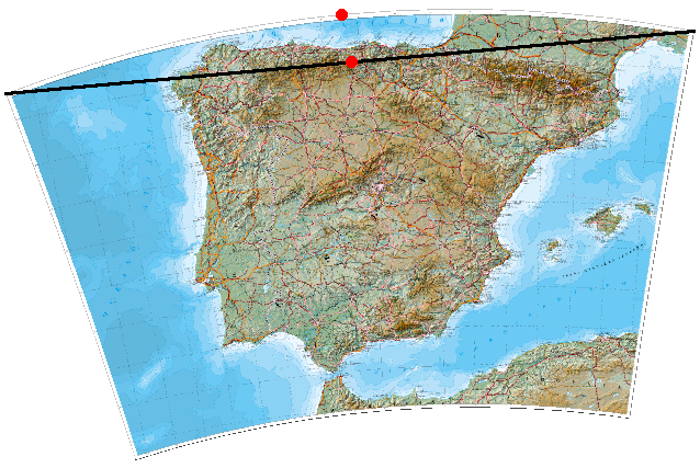
Let’s pick just one of the edges of the map - the top one. Imagine that the map is already projected, and draw an imaginary line between the projected vertices of the edge segment - that’s the black line. The midpoint of the projected vertices is down on the black line, whereas the projected midpoint is the red dot on the top:
And since I’m one of those computer sciencist types who dislikes wasting CPU cycles to add floating point rounding errors, I don’t calculate the distance between those points but, rather, its square.
That squared distance is called the epsilon (ε) of a segment, just because mathematicians like to give the name “epsilon” to pseudo-distances that turn infinitesimally small.
The ε calculation is done for all segments; segments are sorted by their ε; then the segment with the largest ε is selected to be split into two. Splitting a segment splits any triangle that the segment is a part of into two triangles, like so…

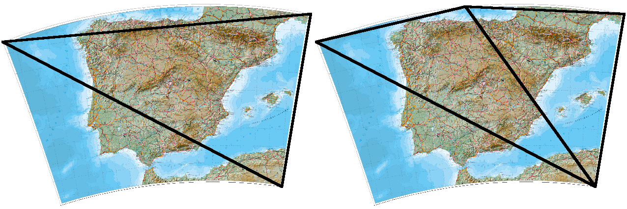
…so with each subdivision, the triangular mesh should fit better the ideally reprojected raster.
Since segments are ordered by their ε, and the segment with the largest ε is destroyed, a priority queue data structure fits perfectly as part of the algorithm. Internally, arrugator uses tinyqueue.
Let’s see how this runs in practice. Arrugator starts with a trivial triangular mesh composed of two adjacent triangles (or, in OpenGL/WebGL parlance, a “quad”). Since arrugator projects all vertices, the initial state looks like:
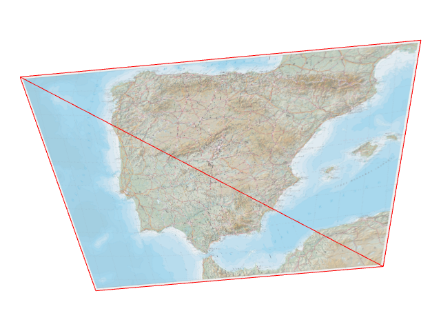
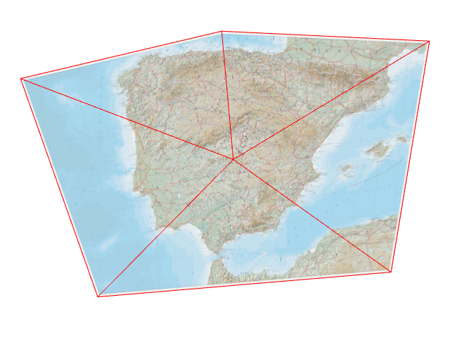
The ε of all five segments is calculated, the segment with the largest ε (which happens to be the diagonal) is selected and triangles are split (and internally, the diagonal gets out of the priority queue, midpoints reprojections are cached, four new segments are added to the priority queue after calculating their εs…)
Select the segment in the queue with the largest ε (which happens to be the top one now), and repeat the process…
…and again.
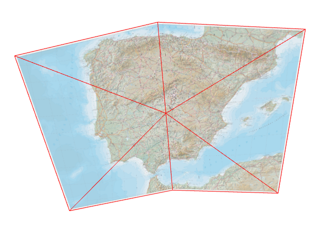
…and again, and again, and again, until ε is lower than the equivalent of 2 pixels:
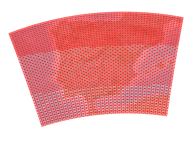
…and again, and again, and again, until ε is lower than the equivalent of half a pixel:
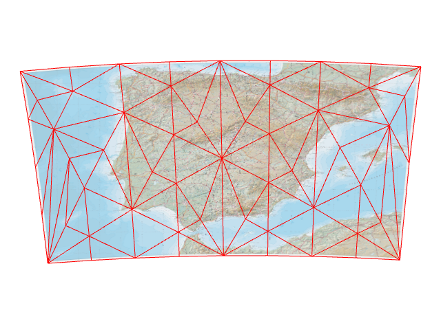
…and five thousand times if we want:
So, there. Arrugator outputs structures in the form of javascript arrays that can be trivially flattened into WebGL-fitting TypedArrays. Since it works with a priority queue, it’s fairly easy to subdivide until needed, and then maybe keep everything in memory for further subdivisions.
On to a couple of technical details. The inputs are:
- A
projectorfunction (which takes anArrayof 2Numbers, and returns anArrayof 2Numbers). Typically this is meant to be aproj4jsforward projection function, likeproj4(srcCRS, destCRS).forward; however, arrugator has no hard dependency on proj4js, so other projection methods could be used. - The unprojected coordinates (an
ArrayofArrays of 2Numbers, typically NW-SW-NE-SE) - The UV-mapping coordinates (an
ArrayofArrays of 2Numbers, typically[[0,0],[0,1],[1,0],[1,1]]) - The vertex indices of the triangles composing the initial mesh (an
ArrayofArrays of 3Numbers, typically[[0,1,3],[0,3,2]]).
Note that the typical input is four vertices, but there’s no hard requirement on that. Any triangular mesh should do (and maybe there are edge cases I haven’t think of where it’s required so things work for weird projections like polyhedral ones).
And the ouputs are:
- The unprojected vertex coordinates (an
ArrayofArrays of 2Numbers) - The projected vertex coordinates (an
ArrayofArrays of 2Numbers) - The UV-mapping coordinates (an
ArrayofArrays of 2Numbers) - The vertex indices of the triangles composing the mesh (an
ArrayofArrays of 3Numbers).
Even though these outputs are not compact TypedArrays, it’s trivial to flatten them and put the data into WebGL attribute&element buffers. In fact, all the image examples above are WebGL visualizations powered by glii.
Using TypedArrays from the beginning is not a viable idea. The goal of this algorithm is to create a triangular mesh with a known upper limit for ε, since the typical use case is to produce a mesh to visualize a raster with an error less than a pixel or a known fraction of a pixel. So the upper limit of ε is known, but the number of subdivisions (and the number of vertices, edge segments and triangles) is unknown until the algorithm runs. This makes it difficult to estimate the size of the data structures, which is a requirement to make this more performant.
In other words: I’m afraid that Vladimir Agafonkin AKA mourner (the one and only rockstar developer) will take this algorithm and redo it so it runs at 865% speed. But I’m not that afraid. Besides, I’m making a best effort to make the algorithm performant.
I’m also slightly afraid that the algorithm might not be the best in terms of computational precision. Avoiding useless square root calculations and subdividing the segments with the higher ε first should avoid computing artifacts (I have been hit by floating point rounding errors in the past), but I have no formal proof that this is the best way. Perhaps subdividing a segment in more than two parts (how many parts given by how large ε is, compared to the desired threshold, might give better -or worse- results).
I’m also confused about the novelty of this algorithm. On one hand, it seems to be a novel algorithm since I haven’t seen any public implementations. On the other hand, it’s so purpose-specific that it might be already implemented and in use, but only behind the scenes. Searching for academic papers on this particular subject is… something I’m not keen on. C’mon, I’m a sci-hub fan and not an academician.
It’s also worth pointing out that, even though the meshes created by arrugator look regular, there is no guarantee of that. Irregular-looking meshes are particularly easy to hit by projecting into EPSG:4326 AKA “WGS84 Equirectangular” (via proj4js):
I have been asked «how does this compare with OpenLayers’ raster reprojection?»
The short answer is «I don’t know».
The long answer is… longer. Arrugator uses forward reprojection only, whereas OpenLayers uses reverse reprojection only. Both have a error threshold, but the meaning of that error threshold might be different. Arrugator enables WebGL, OpenLayers uses 2D canvas (as far as I’m aware). Arrugator can subdivide in smaller triangles at later stages if requested a lower ε threshold (trades higher RAM usage for lower CPU usage); I’m unaware of whether OpenLayers has a similar feature.
This should make for a fun little friendly competition, though.
Arrugator is licensed under the GPLv3. It’s available at a gitlab repo.
Why GPLv3? For me, 2020 has been a year of burnout, and a great deal of it was caused by random people asking for gratis support on my MIT/BSD licensed Leaflet plugins. Besides, there has been an episode of AGPL violation (which was resolved friendly). I’m jaded and tired of publishing stuff under MIT/BSD (which I prefer to call “neoliberal”) licenses.
Anyhow, arrugator is here. This should enable faster raster reprojection visualizations.